

StarC: A Parallel C for Hypercube Computers
Introduction
The C programming language is a product of the DEC PDP-11. C is the way it is because that’s how the PDP-11 worked. ++ and -- exist because the PDP-11 had auto-increment addressing modes. *p++ isn’t a trick; it’s built into the hardware. Strings in C are char arrays with a 0 at the end, because that’s what the PDP-11 did. C has no checks for array bounds because the PDP-11 didn’t check array bounds in hardware. There’s nothing wrong with what C does; like most things it is a product of the material conditions of its development.
StarC is what those material conditions look like for a hypercube.
This language was developed in parallel with a machine with 4,096 RISC-V microcontrollers arranged as a 12-dimensional hypercube. Each processor has 12 neighbors. Communication happens over a time-division multiplexed serial network with deterministic timing. This machine is obviously inspired by the Thinking Machines Connection Machine CM-1. There were two programming languages for the CM-1: C* and *Lisp. Both are dead. The machines that ran these languages are all powered down. If you want to program a hypercube machine in the 21st century, you’re on your own. StarC was created to program this machine.
There are subtle but significant differences between the Connection Machine CM-1 and the machine this language was designed for. The CM-1 had dedicated router ASICs at each node for arbitrary point-to-point communication. This machine doesn’t. It has a TDMA schedule and neighbor links, nothing more. The CM-1 had 1-bit processors with hardware masking for true SIMD execution. This machine has 32-bit RISC-V cores running SPMD, but each processor executes independently. The CM-1 could hide communication latency behind its router. This machine cannot. The network schedule is visible, and communication happens when the schedule says it happens.
These differences shape the language. No router means no get(arbitrary_address). StarC only has neighbor exchange. TDMA means communication is batched into explicit exchange blocks, not scattered through code. SPMD means where is just syntax for if, not a hardware mask operation. The constraints of C* came from the CM-1’s hardware. The constraints of StarC come from this machine’s hardware.
Implementation
In implementation, StarC compiles to C via a Python preprocessor. That’s it. There is no virtual machine or garbage collector or runtime type system. The Python preprocessor rewrites pvar<T>, where, and exchange blocks into C with runtime calls. The runtime handles TDMA timing and communication. There’s no magic, only just enough syntax to express hypercube algorithms without fighting the hardware. C was, and is, a thin wrapper over the PDP-11. StarC is a thin wrapper over a hypercube.
Calling StarC an overcomplication of what could be a bunch of macros is probably correct. However, GCC has no idea about the rules of a hypercube. With StarC, exchange blocks can be validated, there is no accidental dependence on ordering, and no weird multi-superframe behavior. StarC exists to enforce the rules of the machine and illustrate what is possible within the confines of the hardware. Like C did with a PDP-11.
Recommended reading providing context to this specification
Part I: The Machine
Chapter 1: Hardware Model
Before writing StarC code, you need to understand the machine StarC was designed for. StarC was created for exactly one machine: a massively parallel array of microcontrollers that communicate through a hypercube network where messages are passed with a time-division multiplex communications scheme. It is highly recommended you read about the TDMA routing before digging into this.
Dual Networks
The machine has two independent networks:
1. Hypercube Network (TDMA)
The primary communication network. A 12-dimensional hypercube connecting all 4,096 processors. Each processor has 12 neighbors—one per dimension. Communication is time-division multiplexed over a single UART per processor. Deterministic latency: every operation completes in bounded time.
This network handles: neighbor exchange, reductions, scans, broadcasts.
2. Control Tree Network
A hierarchical network separate from the hypercube. The structure is:
- 16 nodes per slice controller
- 16 slice controllers per plane controller
- 16 plane controllers per machine controller
- Machine controller connects to host PC
Physical connections are single-wire serial from slice controllers to nodes. Higher bandwidth than the hypercube for bulk transfers, but variable latency.
This network handles: programming nodes, LED updates, bulk data transfer, host I/O.
                    ┌──────────────┐
                    │    Host PC   │
                    └──────┬───────┘
                           │ USB
                    ┌──────┴───────┐
                    │   Machine    │
                    │  Controller  │
                    └──────┬───────┘
           ┌───────────────┼───────────────┐
           │               │               │
    ┌──────┴──────┐ ┌──────┴──────┐ ┌──────┴──────┐
    │    Plane    │ │    Plane    │ │    Plane    │  (×16)
    │  Controller │ │  Controller │ │  Controller │
    └──────┬──────┘ └──────┬──────┘ └──────┬──────┘
           │               │               │
      ┌────┴────┐     ┌────┴────┐     ┌────┴────┐
      │  Slice  │     │  Slice  │     │  Slice  │     (×16 per plane)
      │Controller│    │Controller│    │Controller│
      └────┬────┘     └────┬────┘     └────┬────┘
           │               │               │
       ┌───┴───┐       ┌───┴───┐       ┌───┴───┐
       │ Nodes │       │ Nodes │       │ Nodes │      (×16 per slice)
       │ 0-15  │       │ 0-15  │       │ 0-15  │
       └───────┘       └───────┘       └───────┘
StarC communication primitives use the hypercube network. Host I/O functions use the control tree.
TDMA Timing
The hypercube network operates on a fixed schedule. Time is divided into phases, and phases are grouped into superframes.
Default timing configuration:
| Parameter | Value |
|---|---|
| Phase clock | 1 kHz |
| Phase duration | 1 ms |
| Phases per superframe | 24 |
| Superframe duration | 24 ms |
| Serial baud rate | 1 Mbps |
| Payload per phase | 80 bytes |
Each of the 12 dimensions gets two phases per superframe: one for each direction. In dimension d, processors with bit d = 0 transmit first, then processors with bit d = 1 transmit. Dimension 0 uses phases 0-1. Dimension 11 uses phases 22-23.
TDMA properties:
- No collisions. Each link has exactly one transmitter per phase. The schedule guarantees this.
- No arbitrary routing. There is no
get(address)orsend(address, value). You cannot send a message to an arbitrary processor. You can only exchange with your 12 hypercube neighbors. - No adaptive forwarding. Packets don’t route around congestion. There is no congestion—the schedule determines everything.
- Multi-hop collectives exist but are implemented as structured tree algorithms over neighbor links, not general routing. A reduction traverses dimensions 0→11 in order, exchanging with neighbors at each step. The path is fixed, not computed per-packet.
Message Framing
Each phase transmits one frame:
┌──────┬────────┬────────┬─────────────────┬───────┐
│ Sync │ Header │ Length │     Payload     │ CRC16 │
│  1B  │   1B   │   1B   │    0-80 B       │  2B   │
└──────┴────────┴────────┴─────────────────┴───────┘
| Field | Size | Description |
|---|---|---|
| Sync | 1 byte | 0xAA — byte alignment |
| Header | 1 byte | Flags and metadata |
| Length | 1 byte | Payload length (0-80) |
| Payload | 0-80 bytes | User data |
| CRC-16 | 2 bytes | Error detection |
At 1 Mbps with 1 ms phases, approximately 100 bytes can transit per phase. After framing overhead and timing margins, 80 bytes of payload remain.
Addressing
The 4,096 processors can be viewed two ways.
Hypercube view: Each processor has a 12-bit address (0-4095). Two processors are neighbors if their addresses differ by exactly one bit. Processor 0x2A3 has neighbors at 0x2A2 (bit 0 differs), 0x2A1 (bit 1 differs), 0x2A7 (bit 2 differs), and so on for all 12 bits.
Grid view: The processors form a 64×64 toroidal grid. Each processor has a row (0-63) and column (0-63). The grid wraps: row 0’s north neighbor is row 63, column 63’s east neighbor is column 0.
These views are equivalent through Gray code mapping:
// Convert grid position to processor ID
int grid_to_pid(int row, int col) {
    int gray_row = row ^ (row >> 1);  // 6-bit Gray code
    int gray_col = col ^ (col >> 1);  // 6-bit Gray code
    return (gray_row << 6) | gray_col;
}
Why Gray code? In Gray code, adjacent values differ by exactly one bit. Moving one step in any cardinal direction—including wrapping at edges—changes exactly one bit of the address. Every NEWS direction is exactly one hypercube hop.
Dimension mapping:
- Bits 0-5 (dimensions 0-5): column position
- Bits 6-11 (dimensions 6-11): row position
- EAST/WEST movement: dimensions 0-5
- NORTH/SOUTH movement: dimensions 6-11
The LED Array
Each processor has one LED. The 64×64 LED matrix maps directly to the 64×64 grid view. Position (row, col) shows the LED of the processor at that grid position.
LEDs are updated via the control tree, not the hypercube network. Setting an LED is a local operation that doesn’t require an exchange block.
Chapter 2: Design Constraints
The CM-1 and this machine are both hypercubes. But they’re built differently, and those differences determine what the programming language can and cannot do.
What the CM-1 Had
Router ASICs. Every CM-1 node had a dedicated routing chip that could accept messages at any time, buffer them, and forward them toward their destination. This enabled arbitrary point-to-point communication. Any processor could send a message to any other processor.
1-bit processors with hardware masking. The CM-1 processors were 1-bit wide and operated in true SIMD fashion. A global instruction stream controlled all processors simultaneously. Hardware masking disabled processors that shouldn’t participate in an operation—they still executed the instruction, but results were discarded.
Hidden latency. The router buffered messages and handled delivery asynchronously. A program could issue a send and continue computing while the router worked.
What This Machine Has Instead
TDMA schedule and neighbor links. No router. Each processor can only talk to its 12 hypercube neighbors, and only during the scheduled phases. There’s no buffering, no forwarding, no arbitrary addressing.
32-bit RISC-V cores running SPMD. Each processor is a full 32-bit microcontroller executing independently. There’s no global instruction stream. Processors run the same program but make independent control flow decisions. “Masking” is just if statements.
Visible latency. Communication happens when the schedule says it happens. If you miss a phase, you wait for the next superframe. The network timing is part of the programming model.
How These Differences Shape the Language
No router → no get(arbitrary_address).
C* and *Lisp had primitives to read from or write to any processor. This requires routing through intermediate nodes. We can’t do that—we have no router. StarC only has neighbor exchange: nbr(dimension, value) swaps values with your neighbor in that dimension. Everything else is built on top of that.
TDMA → explicit exchange blocks.
In C*, you could scatter communication calls throughout your code. The router would handle them whenever. We can’t do that—communication only works during the right phase. StarC batches all communication into explicit exchange blocks. Inside the block, you declare what exchanges you need. The runtime schedules them optimally within the TDMA superframe.
SPMD → where is just if.
In C*, where was a hardware operation that masked processors. Inactive processors still executed but discarded results. In StarC, where is syntactic sugar for if. Each processor independently decides whether to execute the body. There’s no hardware masking—just conditional execution.
Why No Arbitrary Routing?
Building a router is hard. The CM-1’s router was a significant fraction of the machine’s complexity and cost. We don’t have the budget for custom ASICs.
But here’s the thing: most parallel algorithms don’t need arbitrary routing.
| Algorithm | Communication Pattern | Needs Routing? |
|---|---|---|
| Bitonic sort | pid XOR 2^k — hypercube neighbor |
No |
| Parallel prefix | Tree over dimensions | No |
| Reduction | Tree over dimensions | No |
| Stencils | NEWS neighbors | No |
| FFT | Dimension-ordered exchange | No |
| Matrix multiply | Broadcasts + local compute | No |
| Game of Life | 8 neighbors | No |
Bitonic sort is the canonical example. The inner loop exchanges with pid XOR j where j is a power of 2. That’s a single-bit difference—always a hypercube neighbor. The algorithm is topology-aware.
Algorithms that genuinely need arbitrary routing—sparse matrix, irregular graph traversal, hash tables—should use a GPU or a machine with a real interconnect. The hypercube excels at structured, topology-aware communication. StarC supports what the hypercube does well.
Design Principles
These constraints lead to clear design principles:
-
Data is distributed. Each processor has its own data. There’s no shared memory.
-
Operations happen everywhere. When you write
x = x + 1, all 4,096 processors increment their localx. -
Communication is batched. All exchanges go in
exchangeblocks. The runtime schedules them. -
The topology is visible. You know you’re on a hypercube. You know what dimensions cost.
-
Only hypercube-native operations. Neighbor exchange, tree reductions, broadcasts. No arbitrary permutation.
Part II: The Language
Chapter 3: Data Model
This chapter covers how data is represented in StarC: parallel variables, scalars, and processor identity.
Parallel Variables
A pvar<T> is a type qualifier meaning “this value exists once per processor.” In generated code, it’s just a local variable—there’s no distributed shared memory, no magic synchronization. Each of the 4,096 processors has its own independent copy.
pvar<int> x;              // 4,096 integers, one per processor
pvar<float> temperature;  // 4,096 floats
pvar<point_t> position;   // 4,096 structs
When you operate on a pvar, all processors execute the operation simultaneously:
x = 42;           // All 4,096 processors store 42
x = pid();        // Each processor stores its own ID (0-4095)
x = x + 1;        // All processors increment their local x
Initial values are undefined. A freshly declared pvar contains garbage—whatever was in that memory location. Always initialize before use:
pvar<int> x;      // Undefined—could be anything
x = 0;            // Now defined
Scalars
Scalars are ordinary C variables. They have the same value on all processors:
int iterations = 1000;    // Same on all processors
float threshold = 0.001f; // Same on all processors
Scalars are used for control flow (loop counters, convergence flags) and constants. They’re replicated, not distributed.
Mixing scalars and pvars:
pvar<int> x;
int scalar = 100;

x = scalar;          // Every processor stores 100
x = x + scalar;      // Every processor adds 100 to its x
x = x * 2;           // Every processor doubles its x
You cannot assign a pvar to a scalar:
int scalar = x; // ERROR: which processor's x?
To get a scalar from parallel data, use a reduction:
int total = reduce_sum(x);   // Sum across all processors
int maximum = reduce_max(x); // Maximum across all processors
Processor Identity
Every processor knows who it is:
int pid()              // Hypercube address (0-4095)
int coord(int dim)     // Bit 'dim' of the address (0 or 1)
int grid_row()         // Grid row (0-63)
int grid_col()         // Grid column (0-63)
These are how you write position-dependent code:
pvar<int> x;
x = pid();            // Each processor stores its own ID

if (coord(0) == 1) {
    // Only processors with bit 0 set execute this
    // That's processors 1, 3, 5, 7, ... (odd addresses)
}

// Initialize based on grid position
pvar<int> distance_from_center;
int dr = grid_row() - 32;
int dc = grid_col() - 32;
distance_from_center = dr*dr + dc*dc;
Type Limits
Maximum pvar size for exchange: 80 bytes.
This is the payload limit per phase at 1 kHz. If your struct exceeds this, you’ll need to split exchanges or use a slower phase rate.
No pointers in pvars:
pvar<int*> ptr; // ERROR: pointers don't make sense
A pointer on processor 17 pointing to processor 42’s memory is meaningless—there’s no shared address space.
No nested pvars:
pvar<pvar<int>> x; // ERROR: doesn't make sense
Struct Padding
When approaching the 80-byte limit, padding matters:
// Bad: padding wastes space
typedef struct {
    char a;       // 1 byte
    int b;        // 4 bytes (3 bytes padding before)
    char c;       // 1 byte (3 bytes padding after)
} padded_t;       // 12 bytes!

// Good: ordered by size
typedef struct {
    int b;        // 4 bytes
    char a;       // 1 byte
    char c;       // 1 byte
} packed_t;       // 6 bytes (2 bytes trailing padding)

// Best: explicit packing
typedef struct __attribute__((packed)) {
    int b;
    char a;
    char c;
} tight_t;        // 6 bytes, no padding
Order struct members from largest to smallest, or use __attribute__((packed)) when you need precise control.
Arrays of Pvars
Arrays of pvars create multiple values per processor:
pvar<int> buffer[256];    // Each processor has 256 integers
                          // Total: 4,096 × 256 = 1M integers
Indexing works as expected:
pvar<int> A[100];
int i = 50;               // Scalar index

A[i] = pid();             // All processors write to their A[50]

pvar<int> j = pid() % 100;  // Parallel index
pvar<int> val = A[j];       // Each processor reads a different element
Chapter 4: Control Flow
StarC distinguishes between uniform and divergent control flow. This distinction matters because exchange blocks require all processors to participate together.
Two-Phase Execution
StarC programs alternate between two phases:
Compute phase: Local operations only. Arithmetic, memory access, control flow. No network communication.
data = expensive_math(data);
if (data > threshold) data = threshold;
local_array[i] = data;
Exchange phase: Network communication. Batched into explicit exchange blocks.
exchange {
    neighbor = nbr(0, data);
    total = reduce_sum(data);
}
The rhythm is: compute, exchange, compute, exchange. This matches the hardware: the MCU computes, then waits for the TDMA schedule to move data.
Uniform Control Flow
Uniform control flow means all processors take the same path. The condition is a scalar—same value on all processors.
int threshold = 100;          // Scalar—same everywhere

if (threshold > 50) {         // All processors take this branch
    data = data * 2;          // All processors execute this
}

for (int i = 0; i < 10; i++) { // Scalar loop counter
    // All processors execute this loop 10 times
}
Exchange blocks are allowed inside uniform control flow:
for (int iter = 0; iter < 1000; iter++) {  // Scalar bound
    exchange {
        n = news(NORTH, temp);             // All processors participate
    }
    temp = update(temp, n);
}
Divergent Control Flow
Divergent control flow means processors take different paths. The condition is a pvar—different value on each processor.
StarC uses where for divergent control flow:
pvar<int> x;

where (x > 100) {             // Some processors execute, others don't
    x = 0;                    // Only where condition is true
}
Each processor independently evaluates x > 100 and decides whether to execute the body.
if vs where:
if (scalar_condition)— uniform, all processors same branchwhere (pvar_condition)— divergent, per-processor decision
This distinction is enforced. If you write if (pvar_condition), the preprocessor warns you. Use where to signal divergent intent.
Exchange blocks are NOT allowed inside where:
where (x > 0) {
    exchange {                // ERROR: divergent exchange
        y = nbr(0, x);
    }
}
This is illegal because some processors would skip the exchange. The TDMA schedule requires all processors to participate—if half the processors don’t transmit during their phase, communication breaks.
Solution: make data conditional, not exchange:
pvar<int> to_send = (x > 0) ? x : 0;  // Conditional data
exchange {
    y = nbr(0, to_send);              // All processors participate
}
Nesting
Uniform inside uniform: fine.
for (int i = 0; i < 10; i++) {
    if (i % 2 == 0) {
        // All processors, on even iterations
    }
}
Divergent inside divergent: fine.
where (x > 0) {
    where (x > 100) {
        x = 100;              // Only where x > 100
    }
}
Divergent inside uniform: fine.
for (int i = 0; i < 10; i++) {
    where (x > i) {
        x = x - 1;            // Per-processor conditional
    }
}
Uniform with exchange inside divergent: not allowed.
where (x > 0) {
    for (int i = 0; i < 10; i++) {
        exchange { ... }      // ERROR: inside divergent
    }
}
Functions
Functions can take pvar parameters and use where:
pvar<float> clamp(pvar<float> x, float lo, float hi) {
    pvar<float> result = x;
    where (x < lo) { result = lo; }
    where (x > hi) { result = hi; }
    return result;
}

pvar<float> data;
data = clamp(data, 0.0f, 1.0f);  // All processors call simultaneously
Rules for functions:
- All processors call the function together (SPMD)
whereinside functions works normally- No
exchangeblocks inside functions—move them to the caller
The no-exchange rule keeps function semantics simple. A function is pure local computation. Communication happens at the call site.
Chapter 5: Communication
All communication happens inside exchange blocks. This chapter covers the exchange block mechanics and each communication primitive.
Exchange Blocks
An exchange block declares what communications are needed. It’s not sequential code—it’s a declaration that the runtime executes optimally.
exchange {
    a = nbr(0, x);
    b = nbr(5, y);
    total = reduce_sum(z);
}
Snapshot semantics: All input values are captured at block entry. You cannot use the result of one exchange as input to another within the same block.
pvar<int> x = 5;
exchange {
    a = nbr(0, x);    // Captures x=5
    b = nbr(1, x);    // Also captures x=5, not 'a'
}
// Now a and b are valid
Rules:
- Communication primitives may ONLY appear inside
exchangeblocks - No using results from the same block as inputs
- No nested
exchangeblocks - No
exchangeinsidewhereblocks - Scalar control flow (loops with scalar bounds) IS allowed
Scalar loops in exchange blocks:
exchange {
    for (int d = 0; d < 12; d++) {
        neighbors[d] = nbr(d, data);
    }
}
This is allowed because the loop counter is scalar—it’s just syntactic sugar for 12 declarations. The rule is: scalar control flow that can be unrolled at compile time is allowed.
Capacity limit: If declared exchanges exceed one superframe’s capacity, the runtime aborts with an error. This is deliberate—automatic splitting would hide costs and make performance unpredictable. If you need more, use multiple exchange blocks.
Neighbor Exchange: nbr()
T nbr(int dim, T value)
Exchange value with your hypercube neighbor in dimension dim (0-11). Returns the neighbor’s value.
exchange {
    pvar<int> n0 = nbr(0, data);   // Dimension 0 neighbor
    pvar<int> n5 = nbr(5, data);   // Dimension 5 neighbor
}
Your neighbor in dimension dim is the processor whose address differs from yours in bit dim. If you’re processor 0b101010, your dimension-0 neighbor is 0b101011, your dimension-1 neighbor is 0b101000, etc.
Cost: 2 phases per dimension (one each direction).
Grid Neighbors: news()
T news(direction_t dir, T value)
Exchange with your grid neighbor. Directions: NORTH, EAST, SOUTH, WEST.
exchange {
    n = news(NORTH, temp);
    e = news(EAST, temp);
    s = news(SOUTH, temp);
    w = news(WEST, temp);
}
news() is nbr() with automatic dimension selection. The runtime computes which dimension corresponds to each direction based on your grid position and the Gray code mapping.
Edge behavior: The grid wraps toroidally. Row 0’s NORTH neighbor is row 63. Column 63’s EAST neighbor is column 0. Because of Gray code, edge wrapping is still a single-bit change—one hypercube hop.
Cost: NORTH and SOUTH use row dimensions (6-11). EAST and WEST use column dimensions (0-5). These don’t overlap, so four cardinal directions use 8 phases (4 dimensions × 2 phases each).
Diagonal Neighbors
Diagonal neighbors (NE, NW, SE, SW) require two hops: one row dimension and one column dimension. Since exchange blocks can’t use results as inputs within the same block, diagonals need two exchange blocks:
pvar<int> n, e, s, w;
pvar<int> ne, nw, se, sw;

// First: get cardinal neighbors
exchange {
    n = news(NORTH, cell);
    e = news(EAST, cell);
    s = news(SOUTH, cell);
    w = news(WEST, cell);
}

// Second: get diagonals via cardinals
exchange {
    ne = news(NORTH, e);  // My N neighbor's E = my NE
    nw = news(NORTH, w);  // My N neighbor's W = my NW
    se = news(SOUTH, e);  // My S neighbor's E = my SE
    sw = news(SOUTH, w);  // My S neighbor's W = my SW
}
How this works: After the first exchange, I have my east neighbor’s value in e. In the second exchange, news(NORTH, e) sends my e northward. I receive my north neighbor’s e—which is their east neighbor’s value. My north neighbor’s east neighbor is my northeast neighbor.
Cost: Two superframes for 8-neighbor stencils.
Reductions
T reduce_sum(pvar<T> value)
T reduce_min(pvar<T> value)
T reduce_max(pvar<T> value)
T reduce_and(pvar<T> value)
T reduce_or(pvar<T> value)
Combine values from all 4,096 processors into a single scalar. Every processor receives the same result.
exchange {
    int total = reduce_sum(local_count);
    int any_active = reduce_or(is_active);
}
// total and any_active are the same on all processors
Implementation: Tree reduction over 12 dimensions, dimension 0 first, ascending. Each step exchanges with the neighbor in that dimension and combines. After 12 steps, everyone has the global result.
This is a multi-hop operation, but the path is fixed: dimension 0, then 1, then 2, … then 11. It’s a structured tree algorithm, not arbitrary routing.
Floating-point determinism: The dimension ordering is guaranteed and the toolchain enforces -fno-fast-math. Identical inputs always produce identical outputs.
Cost: 24 phases (one full superframe).
Multiple reductions pipeline: Reductions in the same block share the same 24 phases, processing different data streams in parallel:
exchange {
    sum = reduce_sum(x);    // ┐
    max = reduce_max(y);    // ├─ All share one superframe
    count = reduce_sum(1);  // ┘
}
Conditional participation: Processors that shouldn’t contribute use identity values:
// Sum only positive values
pvar<int> contrib = (x > 0) ? x : 0;  // Non-positive → 0
exchange {
    int sum = reduce_sum(contrib);    // Zeros don't affect sum
}
| Operation | Identity Value |
|---|---|
| sum | 0 |
| min | TYPE_MAX |
| max | TYPE_MIN |
| and | ~0 (all 1s) |
| or | 0 |
Scans (Prefix Operations)
pvar<T> scan_sum(pvar<T> value)           // Exclusive
pvar<T> scan_min(pvar<T> value)           // Exclusive
pvar<T> scan_max(pvar<T> value)           // Exclusive
pvar<T> scan_sum_inclusive(pvar<T> value) // Inclusive
pvar<T> scan_min_inclusive(pvar<T> value) // Inclusive
pvar<T> scan_max_inclusive(pvar<T> value) // Inclusive
Prefix operations across all processors.
Exclusive scan: Processor i receives combination of processors 0..i-1 (excluding self).
Inclusive scan: Processor i receives combination of processors 0..i (including self).
pvar<int> x = 1;  // All processors have 1

exchange {
    pvar<int> excl = scan_sum(x);           // Exclusive
    pvar<int> incl = scan_sum_inclusive(x); // Inclusive
}

// Processor 0: excl=0, incl=1
// Processor 1: excl=1, incl=2
// Processor 2: excl=2, incl=3
// ...
// Processor 4095: excl=4095, incl=4096
Scans enable parallel compaction, load balancing, and many classic parallel algorithms.
Cost: 24 phases.
Broadcast
pvar<T> broadcast(int source_pid, T value)
Distribute one processor’s value to all processors.
pvar<float> result;
if (pid() == 0) {
    result = special_computation();
}
exchange {
    pvar<float> everyone = broadcast(0, result);
}
// All processors now have processor 0's result
Semantics: Only the source processor’s value matters. Other processors’ values are undefined—don’t rely on them.
Implementation: Tree distribution over 12 dimensions.
Cost: 24 phases.
Double Buffering
For high MCU utilization, overlap compute with communication:
exchange_async {
    neighbor = nbr(0, data);
}
// MCU computes while FPGA exchanges
next_data = expensive_compute(data);

exchange_wait();  // Block until exchange completes
// Now 'neighbor' is valid
Snapshot semantics: Values are captured when exchange_async begins. Modifying data during compute doesn’t affect what gets sent—the snapshot was already taken.
Rules:
- Cannot read exchange results before
exchange_wait() - Cannot start new
exchange_asyncbefore previousexchange_wait() exchange { }is equivalent toexchange_async { } exchange_wait();
Typical pattern:
// Prime the pipeline
exchange {
    neighbor = nbr(0, data);
}

for (int i = 0; i < 1000; i++) {
    exchange_async {
        neighbor = nbr(0, data);
    }

    // Compute using PREVIOUS neighbor (still valid from last iteration)
    next_data = compute(data, neighbor);

    exchange_wait();
    data = next_data;
}
Chapter 6: Host I/O
Host communication uses the control tree, not the hypercube. This chapter covers loading data, storing results, and debugging output.
Bulk Data Transfer
void load_from_host(pvar<T> *dest, size_t count)
void store_to_host(pvar<T> *src, size_t count)
Load distributes data from the host to all processors. Store collects data from all processors to the host.
pvar<float> input;
load_from_host(&input, 1);   // Each processor gets one float

// ... compute ...

pvar<float> result;
store_to_host(&result, 1);   // Each processor sends one float
Data flows through the control tree: Host → Machine Controller → Plane Controllers → Slice Controllers → Nodes (and reverse for store).
No 80-byte limit. The control tree is a separate network with different constraints. Large transfers are fine:
pvar<float> big_array[1000];
load_from_host(big_array, 1000);  // 4KB per processor—no problem
Latency: Variable, depending on tree traversal and data size. Much slower than hypercube exchange for small data, but higher total bandwidth for bulk transfers.
Console Output
void host_printf(const char *fmt, ...)
Print to the host console. Only processor 0 should call this—other processors’ output is discarded.
if (pid() == 0) {
    host_printf("Starting computation\n");
}

// ... compute and exchange ...

if (pid() == 0) {
    int max = ...;  // result from reduction
    host_printf("Maximum value: %d\n", max);
}
LED Control
void led_set(uint8_t brightness)   // 0 = off, 255 = full
uint8_t led_get(void)              // Read current value
Set this processor’s LED brightness. Updates flow through the control tree to the LED drivers.
// Visualize temperature
led_set((uint8_t)(temperature * 255.0f));

// Binary visualization
led_set(active ? 255 : 0);
LED operations are local—no exchange block needed. All 4,096 processors can set their LEDs simultaneously.
The LED array is a debugging primitive. When something goes wrong, the pattern tells you which processors are affected, which dimensions failed, where data is stuck.
Part III: Programming
Chapter 7: Patterns
The following goes through examples from the StarC Playground, demonstrating the why and how everything in StarC works. Topics covered for each example:
- Mandelbrot Set - Pure compute among 4096 processors
- Plasma - Scalar arrays and SPMD execution
- Dimension Walk - Direct hypercube addressing (
coord(),nbr()on all 12 dimensions) - Bitonic Sort - Topology-aware algorithm (dimension = log₂, hypercube structure dictates algorithm)
- Heat Equation - Stencil operations (
news()), global convergence detection (reduce_max()), conditional participation with identity values - Global Statistics - Pipelined reductions (multiple reduce_* in single exchange block share superframe bandwidth)
- Parallel Prefix - Exclusive vs. inclusive scans (
scan_sum()vsscan_sum_inclusive()) - Stream Compaction - Practical application of prefix sum (computing destination addresses)
- NEWS Blur - Basic 4-neighbor stencil, grid topology (
news()) - Conway’s Game of Life - Complex stencil (8 neighbors via two exchange blocks for diagonals)
- Double-Buffered Stencil - Asynchronous communication (exchange_async/exchange_wait) for overlapping compute and communication
- Random and Pleasing - Embarrassingly parallel computation (replicated scalar state, zero communication, independent per-processor computation)
These examples provide enough context to StarC that you should be able to understand the language after following these examples.
If you’d like to just run these examples, look at the saved examples on the StarC Playground.
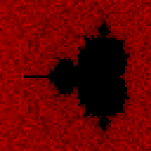
Mandelbrot Set
You’ve seen the Mandelbrot Set. There’s a picture below. You know what I’m talking about here.
If you were to render the Mandelbrot fractal on a single processor, the only way to do it is one pixel at a time. That’s just how it works. But in StarC we have thousands of independent processors. StarC is a language that allows these processors to compute pixels independently. This is that example. There’s no communication here – this is the ‘Hello World’ of SPMD execution. Each processor executes the same code on different data.
// Mandelbrot Set - The Ultimate Embarrassingly Parallel Algorithm!
// Each of the 4,096 processors computes one pixel independently
// No communication needed - pure parallel computation

void main() {
  pvar<int> px = pid() % 64;
  pvar<int> py = pid() / 64;

  // Map to complex plane: Real [-2.5, 1.0], Imaginary [-1.25, 1.25]
  pvar<int> cx = (px * 896) / 64 - 640;  // Fixed-point scale 256
  pvar<int> cy = (py * 640) / 64 - 320;

  pvar<int> zx = cx;
  pvar<int> zy = cy;
  pvar<int> iter = 1;  // Everyone gets at least 1 iteration

  // Iterate z = z² + c up to 32 times
  for (int i = 1; i < 32; i = i + 1) {
    pvar<int> zx2 = (zx * zx) / 256;
    pvar<int> zy2 = (zy * zy) / 256;
    pvar<int> mag_sq = zx2 + zy2;

    // If still bounded (|z|² < 4), count this iteration
    pvar<int> still_bounded = mag_sq < 1024;
    iter = iter + still_bounded;

    // Compute next z = z² + c
    pvar<int> new_zx = zx2 - zy2 + cx;
    pvar<int> new_zy = (2 * zx * zy) / 256 + cy;
    zx = new_zx;
    zy = new_zy;
  }

  // Map iteration count to brightness
  // More iterations = darker (inside set)
  pvar<int> brightness = (32 - iter) * 8;
  led_set(brightness);
}
To describe this code, for this first example I’m going to compare this to serial programming. As in, we have a single microcontroller that’s controlling a 64x64 array of LEDs. The traditional way you render a Mandelbrot set in C looks like this:
  // Serial Mandelbrot - One pixel at a time
  void render_mandelbrot() {
    for (int py = 0; py < 64; py++) {
      for (int px = 0; px < 64; px++) {
        // Map pixel to complex plane
        int cx = (px * 896) / 64 - 640;
        int cy = (py * 640) / 64 - 320;

        // Iterate z = z² + c
        int zx = cx, zy = cy;
        int iter = 1;

        for (int i = 1; i < 32; i++) {
          int zx2 = (zx * zx) / 256;
          int zy2 = (zy * zy) / 256;
          int mag_sq = zx2 + zy2;

          if (mag_sq < 1024) {
            iter++;
            int new_zx = zx2 - zy2 + cx;
            int new_zy = (2 * zx * zy) / 256 + cy;
            zx = new_zx;
            zy = new_zy;
          }
        }

        set_pixel(px, py, (32 - iter) * 8);
      }
    }
  }
Notice the nested loops. There are 64 rows and 64 columns for 4,096 pixels, computed sequentially. If each pixel takes 32 iterations, that 131,072 total iterations before you see the complete image.
In StarC, we eliminate the outer loops entirely. Each processor is a pixel:
  void main() {
    pvar<int> px = pid() % 64;  // I am pixel (px, py)
    pvar<int> py = pid() / 64;

    // Map MY pixel to complex plane
    pvar<int> cx = (px * 896) / 64 - 640;
    pvar<int> cy = (py * 640) / 64 - 320;

    // Compute MY pixel's iteration count
    // ... (same iteration logic)

    led_set(brightness);  // Set MY LED
  }
All 4,096 processors execute this simultaneously. Processor 0 computes pixel (0,0). Processor 1 computes pixel (1,0). Processor 2048 computes pixel (0,32). They all finish after 32 iterations—the same 32 iterations that a single processor would need for one pixel.
How This Works Each processor needs to know which pixel it’s responsible for. The pid() function returns a unique identifier (0-4095), which we decompose into grid coordinates:
pvar<int> px = pid() % 64;  // Column: 0-63
pvar<int> py = pid() / 64;  // Row: 0-63
This creates a per-processor variable—a pvar—that’s different on each processor. Processor 0 gets px=0, py=0. Processor 127 gets px=63, py=1. Processor 4095 gets px=63, py=63.
Next, we map these grid coordinates to the complex plane. The Mandelbrot set lives roughly between -2.5 and +1.0 on the real axis, and -1.25 to +1.25 on the imaginary axis. Since StarC uses integers, we use fixed-point arithmetic with a scale factor of 256:
pvar<int> cx = (px * 896) / 64 - 640;  // Maps [0,63] → [-640, 256]
pvar<int> cy = (py * 640) / 64 - 320;  // Maps [0,63] → [-320, 320]
In fixed-point, -640 represents -2.5 (because -640/256 = -2.5), and 256 represents 1.0. Each processor now has its own complex coordinate c = cx + cy*i.
The Mandelbrot iteration is z = z² + c, starting from z = c. We track how many iterations it takes before |z| > 2 (the point “escapes”):
pvar<int> zx = cx;
pvar<int> zy = cy;
pvar<int> iter = 1;

for (int i = 1; i < 32; i = i + 1) {
  pvar<int> zx2 = (zx * zx) / 256;  // z² in fixed-point
  pvar<int> zy2 = (zy * zy) / 256;
  pvar<int> mag_sq = zx2 + zy2;     // |z|²
}
In traditional code, you’d write if (mag_sq < 1024) to check if the point is still bounded. But in StarC, comparisons return 0 or 1:
pvar<int> still_bounded = mag_sq < 1024;  // 1 if bounded, 0 if escaped
iter = iter + still_bounded;               // Only increment if bounded
Every processor evaluates mag_sq < 1024. For bounded points, still_bounded = 1, so iter increments. For escaped points, still_bounded = 0, so iter stops changing. No branches, no divergence. All 4,096 processors stay in lockstep.
Then we compute the next iteration of z = z² + c using complex arithmetic: (a+bi)² = (a²-b²) + 2abi:
pvar<int> new_zx = zx2 - zy2 + cx;     // Real part
pvar<int> new_zy = (2 * zx * zy) / 256 + cy;  // Imaginary part
zx = new_zx;
zy = new_zy;
After 32 iterations, iter contains the escape count. Points inside the Mandelbrot set never escape, so iter = 32. Points outside escape quickly, so iter might be 1, 2, or 5. We map this to brightness:
pvar<int> brightness = (32 - iter) * 8;
led_set(brightness);
High iter means we’re “inside” the Mandelbrot set, so it’s dark. Low iter means it escaped the Mandelbrot set, so it’s bright.
There’s no communication between processors here. Each processor independently calculates the value of a single pixel. This is the simplest possible parallel program where it’s all the same code, but different data.
This example doesn’t showcase any of StarC’s unique features like exchange(), nbr() or reduce(). There’s no hypercube topology in this code. It could run on any parallel platform. But it does demonstrate that this is a parallel computer. Every pixel completes in 32 iterations. If this were a single processor, the entire graphic would complete in 32 * 4096 iterations. The parallel speedup is 4,096×. It’s faster because it’s parallel.
Plasma
This is a classic demoscene pattern, documented very well on this page. The idea is to create a lava lamp-like pattern across the LED panel. This is a per-CPU compute with no messaging. Like the Mandelbrot example above it’s only an example of a cluster of microcontrollers, not the communication between microcontrollers.

The code is relatively simple, just iterate over four sine waves and plot the amplitude as brightness. The trick for this demo is the scalar array for the sine look up table. This scalar array is saved across all microcontrollers in the cluster:
int sine[256];
  sine[0]=128; sine[1]=131; sine[2]=134; sine[3]=137; sine[4]=140; sine[5]=143; sine[6]=146; sine[7]=149;
  sine[8]=152; sine[9]=155; sine[10]=158; sine[11]=162; sine[12]=165; sine[13]=167; sine[14]=170; sine[15]=173;
  sine[16]=176; sine[17]=179; sine[18]=182; sine[19]=185; sine[20]=188; sine[21]=190; sine[22]=193; sine[23]=196;
  sine[24]=198; sine[25]=201; sine[26]=203; sine[27]=206; sine[28]=208; sine[29]=211; sine[30]=213; sine[31]=215;
  sine[32]=218; sine[33]=220; sine[34]=222; sine[35]=224; sine[36]=226; sine[37]=228; sine[38]=230; sine[39]=232;
  sine[40]=234; sine[41]=235; sine[42]=237; sine[43]=238; sine[44]=240; sine[45]=241; sine[46]=243; sine[47]=244;
The sine lookup table is an artifact of the StarC playground. The actual hardware uses RISC-V cores with floating-point units (roughly ARM Cortex-M3/M4 equivalent), so real StarC programs can use sin() from math.h directly. The StarC Playground, however, is built on JavaScript and doesn’t support math libraries, forcing us to use a lookup table.
This actually gives us a window into olden-time demoscene techniques. Before FPUs were common, this is how the old heads did it. On cheaper microcontrollers without FPUs, this is still how you’d do it today. As a bonus, it also demonstrates the difference between scalar and pvar.
Each microcontroller gets a copy of this array and performs its own lookup while it’s running. The only difference between the microcontrollers is their pid() address, which is used to create the X and Y axes for the display. Consider this an example of, ‘this is just regular C’ along with SPMD programming.
How This Works
The plasma effect combines four sine wave patterns, each varying across space and time:
  pvar<int> v1 = sine[(px * 8 + t * 2) & 255];  // Horizontal waves
  pvar<int> v2 = sine[(py * 8 + t * 3) & 255];  // Vertical waves
  pvar<int> v3 = sine[((px + py) * 6 + t * 2) & 255];  // Diagonal waves
  pvar<int> v4 = sine[(dist + t * 4) & 255];  // Radial waves
Each processor computes its own index into the shared sine[] array using its position (px, py) and the current frame counter (t). The & 255 wraps the index (equivalent to modulo 256) to keep it within the lookup table bounds. All 4,096 processors simultaneously read from the same scalar array, but each with a different index. Processor (0,0) reads sine[frame*2], processor (32,32) reads a completely different entry, and processor (63,63) yet another. The four patterns are averaged together, creating interference patterns that flow and pulse as frame() advances each iteration.
The full listing is available below:
// Classic Demoscene Plasma Effect
// Based on lodev.org/cgtutor/plasma.html
// Combines multiple sine waves for organic flowing patterns

void main() {
  // Sine lookup table (128 = center, range 0-255)
  // Pre-computed: 128 + 127*sin(i * 2*PI / 256)
  int sine[256];
    sine[0]=128; sine[1]=131; sine[2]=134; sine[3]=137; sine[4]=140; sine[5]=143; sine[6]=146; sine[7]=149;
    sine[8]=152; sine[9]=155; sine[10]=158; sine[11]=162; sine[12]=165; sine[13]=167; sine[14]=170; sine[15]=173;
    sine[16]=176; sine[17]=179; sine[18]=182; sine[19]=185; sine[20]=188; sine[21]=190; sine[22]=193; sine[23]=196;
    sine[24]=198; sine[25]=201; sine[26]=203; sine[27]=206; sine[28]=208; sine[29]=211; sine[30]=213; sine[31]=215;
    sine[32]=218; sine[33]=220; sine[34]=222; sine[35]=224; sine[36]=226; sine[37]=228; sine[38]=230; sine[39]=232;
    sine[40]=234; sine[41]=235; sine[42]=237; sine[43]=238; sine[44]=240; sine[45]=241; sine[46]=243; sine[47]=244;
    sine[48]=245; sine[49]=246; sine[50]=248; sine[51]=249; sine[52]=250; sine[53]=250; sine[54]=251; sine[55]=252;
    sine[56]=253; sine[57]=253; sine[58]=254; sine[59]=254; sine[60]=254; sine[61]=255; sine[62]=255; sine[63]=255;
    sine[64]=255; sine[65]=255; sine[66]=255; sine[67]=255; sine[68]=254; sine[69]=254; sine[70]=254; sine[71]=253;
    sine[72]=253; sine[73]=252; sine[74]=251; sine[75]=250; sine[76]=250; sine[77]=249; sine[78]=248; sine[79]=246;
    sine[80]=245; sine[81]=244; sine[82]=243; sine[83]=241; sine[84]=240; sine[85]=238; sine[86]=237; sine[87]=235;
    sine[88]=234; sine[89]=232; sine[90]=230; sine[91]=228; sine[92]=226; sine[93]=224; sine[94]=222; sine[95]=220;
    sine[96]=218; sine[97]=215; sine[98]=213; sine[99]=211; sine[100]=208; sine[101]=206; sine[102]=203; sine[103]=201;
    sine[104]=198; sine[105]=196; sine[106]=193; sine[107]=190; sine[108]=188; sine[109]=185; sine[110]=182; sine[111]=179;
    sine[112]=176; sine[113]=173; sine[114]=170; sine[115]=167; sine[116]=165; sine[117]=162; sine[118]=158; sine[119]=155;
    sine[120]=152; sine[121]=149; sine[122]=146; sine[123]=143; sine[124]=140; sine[125]=137; sine[126]=134; sine[127]=131;
    sine[128]=128; sine[129]=124; sine[130]=121; sine[131]=118; sine[132]=115; sine[133]=112; sine[134]=109; sine[135]=106;
    sine[136]=103; sine[137]=100; sine[138]=97; sine[139]=93; sine[140]=90; sine[141]=88; sine[142]=85; sine[143]=82;
    sine[144]=79; sine[145]=76; sine[146]=73; sine[147]=70; sine[148]=67; sine[149]=65; sine[150]=62; sine[151]=59;
    sine[152]=57; sine[153]=54; sine[154]=52; sine[155]=49; sine[156]=47; sine[157]=44; sine[158]=42; sine[159]=40;
    sine[160]=37; sine[161]=35; sine[162]=33; sine[163]=31; sine[164]=29; sine[165]=27; sine[166]=25; sine[167]=23;
    sine[168]=21; sine[169]=20; sine[170]=18; sine[171]=17; sine[172]=15; sine[173]=14; sine[174]=12; sine[175]=11;
    sine[176]=10; sine[177]=9; sine[178]=7; sine[179]=6; sine[180]=5; sine[181]=5; sine[182]=4; sine[183]=3;
    sine[184]=2; sine[185]=2; sine[186]=1; sine[187]=1; sine[188]=1; sine[189]=0; sine[190]=0; sine[191]=0;
    sine[192]=0; sine[193]=0; sine[194]=0; sine[195]=0; sine[196]=1; sine[197]=1; sine[198]=1; sine[199]=2;
    sine[200]=2; sine[201]=3; sine[202]=4; sine[203]=5; sine[204]=5; sine[205]=6; sine[206]=7; sine[207]=9;
    sine[208]=10; sine[209]=11; sine[210]=12; sine[211]=14; sine[212]=15; sine[213]=17; sine[214]=18; sine[215]=20;
    sine[216]=21; sine[217]=23; sine[218]=25; sine[219]=27; sine[220]=29; sine[221]=31; sine[222]=33; sine[223]=35;
    sine[224]=37; sine[225]=40; sine[226]=42; sine[227]=44; sine[228]=47; sine[229]=49; sine[230]=52; sine[231]=54;
    sine[232]=57; sine[233]=59; sine[234]=62; sine[235]=65; sine[236]=67; sine[237]=70; sine[238]=73; sine[239]=76;
    sine[240]=79; sine[241]=82; sine[242]=85; sine[243]=88; sine[244]=90; sine[245]=93; sine[246]=97; sine[247]=100;
    sine[248]=103; sine[249]=106; sine[250]=109; sine[251]=112; sine[252]=115; sine[253]=118; sine[254]=121; sine[255]=124;

  pvar<int> px = pid() % 64;
  pvar<int> py = pid() / 64;

  for (;;) {
    int t = frame();

    // Classic plasma: combine multiple sine waves
    // Pattern 1: Horizontal waves
    pvar<int> v1 = sine[(px * 6 + t * 2) & 255];

    // Pattern 2: Vertical waves
    pvar<int> v2 = sine[(py * 8 + t * 3) & 255];

    // Pattern 3: Diagonal waves
    pvar<int> v3 = sine[((px + py) * 4 + t * 2) & 255];

    // Pattern 4: Distance from center
    pvar<int> dx = px - 32;
    pvar<int> dy = py - 32;
    pvar<int> dist = (dx * dx + dy * dy) / 12;
    pvar<int> v4 = sine[(dist + t * 4) & 255];

    // Combine all patterns (average)
    pvar<int> brightness = (v1 + v2 + v3 + v4) / 4;

    led_set(brightness);
    barrier();
  }
}
Dimension Walk
Pure hypercube. Uses coord(dim), nbr() across all 12 dimensions.
// Dimension Walk - Hamiltonian path through 12D hypercube
// Uses coord() to build position from dimension bits
// Uses nbr() to highlight the 12-dimensional neighborhood
// Gray code ensures each step moves to exactly 1 neighbor

void main() {
  // Build my position from individual dimension coordinates
  pvar<int> c0 = coord(0);
  pvar<int> c1 = coord(1);
  pvar<int> c2 = coord(2);
  pvar<int> c3 = coord(3);
  pvar<int> c4 = coord(4);
  pvar<int> c5 = coord(5);
  pvar<int> c6 = coord(6);
  pvar<int> c7 = coord(7);
  pvar<int> c8 = coord(8);
  pvar<int> c9 = coord(9);
  pvar<int> c10 = coord(10);
  pvar<int> c11 = coord(11);

  // My 12-bit position: c11 c10 c9 ... c2 c1 c0
  pvar<int> my_position = (c11 << 11) | (c10 << 10) | (c9 << 9) | (c8 << 8) |
                          (c7 << 7) | (c6 << 6) | (c5 << 5) | (c4 << 4) |
                          (c3 << 3) | (c2 << 2) | (c1 << 1) | c0;

  int counter = 0;

  for (;;) {
    // Convert counter to Gray code (Hamiltonian path property)
    int gray = counter ^ (counter >> 1);

    // Am I the current position?
    pvar<int> lit = 0;
    where (my_position == gray) {
      lit = 255;  // Bright: current position
    }

    // Use nbr() to highlight my 12 neighbors in the hypercube
    exchange {
      pvar<int> n0 = nbr(0, lit);
      pvar<int> n1 = nbr(1, lit);
      pvar<int> n2 = nbr(2, lit);
      pvar<int> n3 = nbr(3, lit);
      pvar<int> n4 = nbr(4, lit);
      pvar<int> n5 = nbr(5, lit);
      pvar<int> n6 = nbr(6, lit);
      pvar<int> n7 = nbr(7, lit);
      pvar<int> n8 = nbr(8, lit);
      pvar<int> n9 = nbr(9, lit);
      pvar<int> n10 = nbr(10, lit);
      pvar<int> n11 = nbr(11, lit);

      // If any neighbor is bright, I'm dim (shows hypercube connectivity)
      pvar<int> any_neighbor = n0 | n1 | n2 | n3 | n4 | n5 | n6 | n7 | n8 | n9 | n10 | n11;
      where (any_neighbor > 0 && lit == 0) {
        lit = 64;  // Dim: neighbor of current position
      }
    }

    led_set(lit);

    // Advance to next Gray code position
    counter = (counter + 1) & 4095;
    barrier();
  }
}
Bitonic Sort
The canonical hypercube algorithm. nbr(log₂(j), key). Proves topology = algorithm.
Heat Equation
Stencil + convergence. news() for neighbors, reduce_max() for termination. Shows conditional participation with identity values.
Global Statistics
Pipelined reductions. Multiple reduce_* in one exchange block. Shows they share the superframe.
Parallel Prefix (Exclusive and Inclusive)
scan_sum() and scan_sum_inclusive(). Shows the difference.
Stream Compaction
Application of prefix sum. scan_sum() → destination addresses.
NEWS Blur
4-neighbor stencil. Clean news() usage.

// 2D Gaussian blur using NEWS communication
// Each pixel averages with its 4 neighbors

void main() {
  pvar<int> x = pid() % 64;
  pvar<int> y = pid() / 64;

  // Initialize with a simple pattern
  pvar<int> value = 0;
  where (x > 20 && x < 44 && y > 20 && y < 44) {
    value = 255;
  }

  // Declare neighbor variables outside the loop
  pvar<int> north;
  pvar<int> south;
  pvar<int> east;
  pvar<int> west;

  for (;;) {
    // All communication must happen in an exchange block
    exchange {
      north = news(NORTH, value);
      south = news(SOUTH, value);
      east = news(EAST, value);
      west = news(WEST, value);
    }

    // 5-point stencil: average with 4 neighbors
    pvar<int> sum = value * 2 + north + south + east + west;
    value = sum / 6;

    led_set(value);

    barrier();
  }
}
Conway’s Game of Life
Because of course a gigantic LED array needs to run Game of Life. This example uses two iterations of the news() grid to create a stencil with eight neighbors.
// Conway's Game of Life using NEWS communication
// Classic cellular automaton with multiple patterns

void main() {
  pvar<int> x = pid() % 64;
  pvar<int> y = pid() / 64;

  pvar<int> alive = 0;

  // Acorn pattern at (10, 10)
  where ((x == 11 && y == 10) || (x == 13 && y == 11) ||
         (x == 10 && y == 12) || (x == 11 && y == 12) ||
         (x == 14 && y == 12) || (x == 15 && y == 12) ||
         (x == 16 && y == 12)) {
    alive = 1;
  }

  // R-pentomino at (40, 20)
  where ((x == 41 && y == 20) || (x == 42 && y == 20) ||
         (x == 40 && y == 21) || (x == 41 && y == 21) ||
         (x == 41 && y == 22)) {
    alive = 1;
  }

  // Glider at (50, 50)
  where ((x == 50 && y == 50) || (x == 51 && y == 51) ||
         (x == 49 && y == 52) || (x == 50 && y == 52) ||
         (x == 51 && y == 52)) {
    alive = 1;
  }

  // Lightweight spaceship (LWSS) at (5, 40)
  where ((x == 6 && y == 40) || (x == 7 && y == 40) ||
         (x == 8 && y == 40) || (x == 9 && y == 40) ||
         (x == 5 && y == 41) || (x == 10 && y == 41) ||
         (x == 10 && y == 42) || (x == 5 && y == 43) ||
         (x == 9 && y == 43)) {
    alive = 1;
  }

  // Pulsar (oscillator) at (30, 35) - period 3
  where ((x == 28 && y == 29) || (x == 29 && y == 29) ||
         (x == 30 && y == 29) || (x == 34 && y == 29) ||
         (x == 35 && y == 29) || (x == 36 && y == 29)) {
    alive = 1;
  }
  where ((x == 26 && y == 31) || (x == 31 && y == 31) ||
         (x == 33 && y == 31) || (x == 38 && y == 31)) {
    alive = 1;
  }
  where ((x == 26 && y == 32) || (x == 31 && y == 32) ||
         (x == 33 && y == 32) || (x == 38 && y == 32)) {
    alive = 1;
  }
  where ((x == 26 && y == 33) || (x == 31 && y == 33) ||
         (x == 33 && y == 33) || (x == 38 && y == 33)) {
    alive = 1;
  }
  where ((x == 28 && y == 34) || (x == 29 && y == 34) ||
         (x == 30 && y == 34) || (x == 34 && y == 34) ||
         (x == 35 && y == 34) || (x == 36 && y == 34)) {
    alive = 1;
  }
  where ((x == 28 && y == 39) || (x == 29 && y == 39) ||
         (x == 30 && y == 39) || (x == 34 && y == 39) ||
         (x == 35 && y == 39) || (x == 36 && y == 39)) {
    alive = 1;
  }
  where ((x == 26 && y == 40) || (x == 31 && y == 40) ||
         (x == 33 && y == 40) || (x == 38 && y == 40)) {
    alive = 1;
  }
  where ((x == 26 && y == 41) || (x == 31 && y == 41) ||
         (x == 33 && y == 41) || (x == 38 && y == 41)) {
    alive = 1;
  }
  where ((x == 26 && y == 42) || (x == 31 && y == 42) ||
         (x == 33 && y == 42) || (x == 38 && y == 42)) {
    alive = 1;
  }
  where ((x == 28 && y == 44) || (x == 29 && y == 44) ||
         (x == 30 && y == 44) || (x == 34 && y == 44) ||
         (x == 35 && y == 44) || (x == 36 && y == 44)) {
    alive = 1;
  }

  // Declare neighbor variables outside the loop
  pvar<int> n;
  pvar<int> s;
  pvar<int> e;
  pvar<int> w;
  pvar<int> ne;
  pvar<int> nw;
  pvar<int> se;
  pvar<int> sw;

  for (;;) {

    // Exchange 1: Get cardinal neighbors
    exchange {
      n = news(NORTH, alive);
      s = news(SOUTH, alive);
      e = news(EAST, alive);
      w = news(WEST, alive);
    }

    // Exchange 2: Get diagonal neighbors via cardinals
    // My north neighbor's east = my northeast
    exchange {
      ne = news(NORTH, e);
      nw = news(NORTH, w);
      se = news(SOUTH, e);
      sw = news(SOUTH, w);
    }

    pvar<int> neighbors = n + s + e + w + ne + nw + se + sw;

    // Conway's rules (optimized):
    // Live cell: survives if 2-3 neighbors
    // Dead cell: born if exactly 3 neighbors
    pvar<int> survive = (alive == 1) && (neighbors == 2 || neighbors == 3);
    pvar<int> born = (alive == 0) && (neighbors == 3);
    alive = survive || born;

    // Display: compute LED value directly (faster than where blocks)
    pvar<int> brightness = alive * 255;
    led_set(brightness);

    barrier();
  }
}
Double-Buffered Stencil
exchange_async / exchange_wait. MCU utilization.
Random and Pleasing
This is the single reason you’ve ever seen a Connection Machine in print or media. The original Connection Machines all had a, “Random and Pleasing” setting for the front lights. You can see it in Jurassic Park. There’s some discussion over what Random and Pleasing actually is - here’s Trammell Hudson’s blog - and after spending far too much time on this project I believe this may actually be a representation of the CM-5’s Random and Pleasing mode. I’m sure Danny or Tamiko or someone will eventually email me and tell me what all the ‘demo modes’ on all iterations of the Connection Machine actually do. I’ll update that here.
For my machine’s Random and Pleasing mode, I break up the 64x64 pixel panel into 1x16 ‘windows’. These windows either scroll left or right. The content of these windows is determined by an LFSR – a pseudo-random bit generator. A bit is generated from the LFSR, and pushed into the ‘window’. Another bit is generated by the LFSR (either 1 or 0), and the existing bit in each window is pushed to the left or right. The eventual result is a “shimmer” of LEDs. It looks like the computer is doing something important.
This Random and Pleasing mode is enough like the original mode found in Connection Machines that I’ll call it a clone. It’s not a direct copy, but then again the layout of the front panel isn’t either.
How this works
First, we define 8 LFSRs shared across all the processors. Then, we create some ‘bookkeeping’ variables per processor. These bookkeeping variables define the x and y locations on the display. The display is split up into four ‘columns’ consisting of 1x16 pixel ‘windows’, so we declare those as well.
  int lfsr[8];
  lfsr[0] = 0xACE1BEEF;
  ...
  lfsr[7] = 0xBADC0FFE;

  // Per-processor state: figure out my role
  pvar<int> x = pid() % 64;
  pvar<int> y = pid() / 64;
  pvar<int> col = x / 16;           // Column (0-3)
  pvar<int> pixel_in_col = x % 16;  // Pixel within window (0-15)
  pvar<int> segment_id = y * 4 + col;  // Window ID (0-255)
Next, we assign each window a unique LFSR bit. Each window will scroll randomly left or right, so we create the direction with some bitshift trickery:
  // Assign each window a unique LFSR bit (8 LFSRs × 32 bits = 256)
  pvar<int> permuted = (segment_id * 131 + 73) & 0xFF;
  pvar<int> my_lfsr_idx = permuted / 32;  // Which LFSR (0-7)
  pvar<int> my_bit_pos = permuted % 32;   // Which bit (0-31)

  // Pseudo-random scroll direction per window
  pvar<int> my_direction = ((segment_id * 179 + 41) >> 3) & 1;
Now comes the main loop, and this is where StarC reveals its elegance. The infinite loop steps all 8 LFSRs using a plain C for-loop—this executes once per frame, not per processor. Each LFSR advances using Galois LFSR logic with the primitive polynomial x³² + x³¹ + x²⁹ + x¹ + 1:
    for (int i = 0; i < 8; i++) {
      int lsb = lfsr[i] & 1;
      lfsr[i] = (lfsr[i] >> 1) ^ ((-lsb) & 0xA0000002);
    }
Then the magic happens: each of the 4096 processors simultaneously reads from the scalar LFSR array using its own index: lfsr[my_lfsr_idx]. This single line demonstrates massively parallel array access—256 different windows extracting 256 different bits from 8 LFSRs, all at once:
pvar<int> new_bit = (lfsr[my_lfsr_idx] >> my_bit_pos) & 1;
Each processor maintains its own 16-bit scroll buffer. The where() blocks handle directional scrolling—processors with my_direction == 0 shift right (pushing new bits from the left), while processors with my_direction == 1 shift left. Notice there’s zero communication between processors; this is embarrassingly parallel:
    where (my_direction == 0) {
      scroll_buffer = (scroll_buffer >> 1) | (new_bit << 15);
    }
    where (my_direction == 1) {
      scroll_buffer = (scroll_buffer << 1) | new_bit;
    }
Finally, each processor extracts its display bit from its scroll buffer based on its position within the window, and sets its LED intensity. The barrier() synchronizes all processors before the next frame:
    pvar<int> display_bit = (scroll_buffer >> pixel_in_col) & 1;
    led_set(display_bit * 255);
    barrier();
The result is 256 independent windows, each scrolling its own LFSR-generated pattern in its own direction, creating the “thinking computer” shimmer. This is StarC’s design philosophy in action: it’s just C until it isn’t. Plain for-loops stepping LFSRs in scalar context, then massively parallel array indexing when you need it.
Code Listing
// LFSR Scrolling Columns - Embarrassingly Parallel!
// 64 rows × 4 columns = 256 independent 16-pixel-wide windows
// Each window displays a 16-bit LFSR scroll buffer, scrolling left/right
// Based on real hardware implementation (animations.h)

void main() {
  // Scalar array: 8 LFSRs shared across all processors
  // Polynomial: x^32 + x^31 + x^29 + x^1 + 1 → mask 0xA0000002
  int lfsr[8];
  lfsr[0] = 0xACE1BEEF;
  lfsr[1] = 0xCAFEDEAD;
  lfsr[2] = 0x12345678;
  lfsr[3] = 0x9ABCDEF0;
  lfsr[4] = 0xFEDCBA98;
  lfsr[5] = 0x76543210;
  lfsr[6] = 0xDEADBEEF;
  lfsr[7] = 0xBADC0FFE;

  // Per-processor state: figure out my role
  pvar<int> x = pid() % 64;
  pvar<int> y = pid() / 64;
  pvar<int> col = x / 16;           // Column (0-3)
  pvar<int> pixel_in_col = x % 16;  // Pixel within window (0-15)
  pvar<int> segment_id = y * 4 + col;  // Window ID (0-255)

  // Assign each window a unique LFSR bit (8 LFSRs × 32 bits = 256)
  pvar<int> permuted = (segment_id * 131 + 73) & 0xFF;
  pvar<int> my_lfsr_idx = permuted / 32;  // Which LFSR (0-7)
  pvar<int> my_bit_pos = permuted % 32;   // Which bit (0-31)

  // Pseudo-random scroll direction per window
  pvar<int> my_direction = ((segment_id * 179 + 41) >> 3) & 1;

  // Each window has a 16-bit scroll buffer
  pvar<int> scroll_buffer = 0;

  for (;;) {
    // Step all 8 LFSRs (plain C loop)
    for (int i = 0; i < 8; i++) {
      int lsb = lfsr[i] & 1;
      lfsr[i] = (lfsr[i] >> 1) ^ ((-lsb) & 0xA0000002);
    }

    // Extract my assigned bit - index scalar array with pvar!
    pvar<int> new_bit = (lfsr[my_lfsr_idx] >> my_bit_pos) & 1;

    // Shift into scroll buffer (direction depends on my_direction)
    where (my_direction == 0) {
      scroll_buffer = (scroll_buffer >> 1) | (new_bit << 15);
    }
    where (my_direction == 1) {
      scroll_buffer = (scroll_buffer << 1) | new_bit;
    }

    // Display my bit from the scroll buffer
    pvar<int> display_bit = (scroll_buffer >> pixel_in_col) & 1;
    led_set(display_bit * 255);

    barrier();
  }
}
Chapter 8: Performance
This chapter explains the cost model and how to reason about performance.
Timing Model
At 1 kHz phase clock:
| Unit | Duration |
|---|---|
| Phase | 1 ms |
| Superframe (24 phases) | 24 ms |
Operation costs:
| Operation | Phases | Time |
|---|---|---|
nbr() — one dimension |
2 | 2 ms |
nbr() — all 12 dimensions |
24 | 24 ms |
news() — 4 cardinal directions |
8 | 8 ms |
reduce_*() — one or more |
24 | 24 ms |
scan_*() |
24 | 24 ms |
broadcast() |
24 | 24 ms |
Exchange Scheduling
The runtime schedules exchanges to minimize superframe usage.
What fits in one superframe:
- Up to 12
nbr()calls on different dimensions - AND/OR multiple pipelined reductions
- AND/OR one scan
- AND/OR one broadcast
What exceeds capacity (runtime error):
- More than ~160 bytes total on a single dimension
- Scan + reduction in same block (both need the full tree)
- Too many exchanges overall
Examples:
// OK: 12 different dimensions
exchange {
    for (int d = 0; d < 12; d++) {
        neighbors[d] = nbr(d, data);
    }
}

// OK: multiple reductions (pipelined)
exchange {
    sum = reduce_sum(x);
    max = reduce_max(x);
    min = reduce_min(x);
}

// ERROR: reduction + scan both need full tree
exchange {
    total = reduce_sum(x);
    prefix = scan_sum(y);   // Can't share with reduction
}

// OK: separate blocks
exchange { total = reduce_sum(x); }
exchange { prefix = scan_sum(y); }
Automatic Reordering
The runtime reorders nbr() calls by dimension for optimal phase usage:
exchange {
    d11 = nbr(11, x);  // Declared first
    d0 = nbr(0, y);    // Declared second
    d5 = nbr(5, z);    // Declared third
}
// Executes: d0 (phases 0-1), d5 (phases 10-11), d11 (phases 22-23)
You don’t need to think about phase ordering—just declare what you need.
Bandwidth
| Path | Payload | Bandwidth |
|---|---|---|
| Hypercube (per dimension) | 80 B / 2 ms | 40 KB/s |
| Hypercube (all dimensions) | 960 B / 24 ms | 40 KB/s |
| Control tree (bulk) | Unlimited | ~1 MB/s |
The hypercube is latency-optimized: small payloads, fast phases, deterministic timing. Use it for algorithm communication.
The control tree is bandwidth-optimized: large transfers, variable latency. Use it for bulk I/O.
MCU Utilization
Without double buffering:
During an exchange, the MCU waits. At 133 MHz, a 24 ms superframe wastes 3.2 million cycles.
With double buffering:
The MCU computes iteration N+1 while the FPGA exchanges iteration N. Utilization depends on the ratio:
- If compute > exchange: MCU-bound, utilization ≈ 100%
- If compute < exchange: exchange-bound, utilization ≈ compute/exchange
- If compute ≈ exchange: optimal overlap, utilization ≈ 100%
Phase Rate Trade-offs
The phase rate is configurable:
| Rate | Superframe | Payload/Phase | Use Case |
|---|---|---|---|
| 100 Hz | 240 ms | 800 bytes | Debug, huge payloads |
| 1 kHz | 24 ms | 80 bytes | Default, balanced |
| 10 kHz | 2.4 ms | 8 bytes | Low latency, small data |
Slower rates give more payload per phase. Faster rates give lower latency but smaller payloads.
Iteration Rates
Typical workloads at 1 kHz:
| Workload | Exchange Time | Iter/Sec |
|---|---|---|
| 4-neighbor stencil | ~8 ms | ~100 |
| 8-neighbor stencil | ~48 ms | ~20 |
| Stencil + reduction | ~32 ms | ~30 |
| Single bitonic step | ~2 ms | ~500 |
Part IV: Implementation
Chapter 9: Toolchain
This chapter describes how StarC source code becomes executable firmware.
Build Pipeline
algorithm.starc
      ↓
  starc_pp.py (Python preprocessor)
      ↓
algorithm.c (plain C with runtime calls)
      ↓
  gcc / riscv-gcc
      ↓
algorithm.elf (executable)
StarC is not a compiler. It’s a preprocessor that rewrites StarC syntax into C, then a standard C compiler produces the binary.
Preprocessor Transformations
The preprocessor tokenizes the source (not regex—proper tokenization) and rewrites StarC constructs:
| StarC | Generated C |
|---|---|
pvar<T> x; |
T x; |
where (c) { } |
if (c) { } |
if (c) { } |
if (c) { } (validated: c must be scalar) |
exchange { ... } |
star_ex_begin(); ... star_ex_execute(); |
exchange_async { ... } |
star_ex_begin(); ... star_ex_start(); |
exchange_wait() |
star_ex_wait(); |
nbr(d, v) |
star_ex_nbr(d, &r, &v, sizeof(v)) |
reduce_sum(v) |
star_ex_reduce(SUM, &r, &v, sizeof(v)) |
scan_sum(v) |
star_ex_scan(SUM, EXCL, &r, &v, sizeof(v)) |
news(NORTH, v) |
star_ex_news(NORTH, &r, &v, sizeof(v)) |
pid() |
star_pid() |
grid_row() |
star_grid_row() |
grid_col() |
star_grid_col() |
Preprocessor Diagnostics
The preprocessor validates StarC rules and emits warnings/errors:
- Warning:
ifcondition appears to involve a pvar (should usewhere) - Error:
exchangeblock insidewhereblock - Error: Exchange result used as input within same block
- Error: Nested
exchangeblocks - Error: Communication primitive outside
exchangeblock - Error: Cannot assign pvar to scalar variable
- Catches
scalar = pvar_valueassignments - This is a type error that breaks SPMD semantics
- Catches
- Error: Cannot mutate scalar variable inside where() block
- Catches
where (cond) { scalar = scalar + 1; } - Prevents the “4096 decrements per frame” bug class
- Catches
- Error: Array index out of bounds
- Runtime bounds checking for scalar arrays
arr[10]when array has length 3
Things that we’re not catching (for now) that we probably should
- Warning: For-loop with
pvarcondition:for (int i = 0; i < my_pvar; i++)is a non-deterministic iteration count ` This should probably be an error
- Warning: Uninitialized
pvarreadpvar<int> x; led_set(x);- x could be undefined
- Error: Scalar declared inside loop
for (;;) { int counter = 0; }- re-declares every frame- Should be caught
- Error: Array subscript with non-integer
arr[1.5]orarr[pvar_value](the second is actually legal!)- We allow pvar subscripts for
lfsr[my_lfsr_idx]
Compiler Settings
The toolchain enforces specific compiler settings:
-fno-fast-math— guarantees floating-point reproducibility in reductions/scans- Standard optimization flags as appropriate for the target
Backends
Simulator backend:
Compiles to run on desktop with N virtual processors (configurable, typically 16 or 64 for testing). Used for debugging and algorithm development.
./starc_pp.py src/algorithm.starc -o build/algorithm.c
gcc -DSTAR_SIM -Ilibstar build/algorithm.c libstar/sim_backend.c -o build/sim
./build/sim
Hardware backend:
Compiles for actual RISC-V nodes. Links against TDMA runtime.
./starc_pp.py src/algorithm.starc -o build/algorithm.c
riscv-gcc -DSTAR_HW -Ilibstar build/algorithm.c libstar/hw_backend.c -o build/firmware.elf
Chapter 10: Runtime
This chapter describes the runtime library and hardware interface.
Exchange Block Compilation
The preprocessor transforms an exchange block into runtime calls:
exchange {
    a = nbr(0, x);
    b = nbr(5, y);
    total = reduce_sum(z);
}
Becomes:
{
    star_ex_t __ex;
    star_ex_begin(&__ex);

    star_ex_nbr(&__ex, 0, &a, &x, sizeof(x));
    star_ex_nbr(&__ex, 5, &b, &y, sizeof(y));
    star_ex_reduce(&__ex, STAR_SUM, &total, &z, sizeof(z));

    star_ex_execute(&__ex);  // Blocks until complete
}
The star_ex_t structure collects exchange declarations. star_ex_execute() validates capacity, schedules phases, and executes.
FPGA Interface
The MCU communicates with the FPGA via memory-mapped registers:
| Address | Register | Description |
|---|---|---|
| 0x4000_0000 | PHASE_COUNTER | Current phase (0-23) |
| 0x4000_0004 | PHASE_CONFIG | Phase clock divider |
| 0x4000_0008 | TX_DATA | Transmit FIFO |
| 0x4000_000C | RX_DATA | Receive FIFO |
| 0x4000_0010 | TX_STATUS | TX FIFO status |
| 0x4000_0014 | RX_STATUS | RX FIFO status |
| 0x4000_0018 | DIM_SELECT | Current dimension (pin mux) |
| 0x4000_001C | FRAME_COUNT | Superframes since reset |
| 0x4000_0020 | ERROR_COUNT | CRC errors per dimension |
Phase Rate Configuration
void star_set_phase_rate(int hz);
Sets the FPGA’s phase clock divider. Valid values: 100, 1000, 10000.
| Rate | Superframe | Payload |
|---|---|---|
| 100 Hz | 240 ms | 800 B |
| 1 kHz | 24 ms | 80 B |
| 10 kHz | 2.4 ms | 8 B |
Error Handling
CRC errors:
Each received frame is CRC-checked. On failure:
- Error counter for that dimension increments
- Payload is zeroed
- Execution continues
Query errors:
int star_crc_errors(int dim);  // Errors on dimension dim
void star_clear_errors(void);  // Reset all counters
Capacity exceeded:
If an exchange block declares more than fits in one superframe, the runtime aborts with an error message. This is deliberate—automatic splitting would hide costs.
Desynchronization:
If the TDMA clock drifts or a processor crashes, the watchdog timer triggers a hardware reset. There is no automatic recovery.
Appendices
Appendix A: Quick Reference
Types and Identity
pvar<T>              // Parallel variable (one per processor)
int pid()            // Processor ID (0-4095)
int coord(int dim)   // Bit 'dim' of address (0 or 1)
int grid_row()       // Grid row (0-63)
int grid_col()       // Grid column (0-63)
Communication (exchange blocks only)
// Neighbor exchange
T nbr(int dim, T val)              // Hypercube neighbor
T news(dir, T val)                 // Grid neighbor (N/E/S/W)

// Reductions → scalar
T reduce_sum(pvar<T>)
T reduce_min(pvar<T>)
T reduce_max(pvar<T>)
T reduce_and(pvar<T>)
T reduce_or(pvar<T>)

// Scans → pvar
pvar<T> scan_sum(pvar<T>)              // Exclusive
pvar<T> scan_min(pvar<T>)              // Exclusive
pvar<T> scan_max(pvar<T>)              // Exclusive
pvar<T> scan_sum_inclusive(pvar<T>)    // Inclusive
pvar<T> scan_min_inclusive(pvar<T>)    // Inclusive
pvar<T> scan_max_inclusive(pvar<T>)    // Inclusive

// Broadcast
pvar<T> broadcast(int source, T val)
Control
if (scalar_cond) { }     // Uniform (all same branch)
where (pvar_cond) { }    // Divergent (per-processor)
exchange { }             // Synchronous communication
exchange_async { }       // Asynchronous communication
exchange_wait()          // Wait for async
barrier()                // Global sync (rarely needed)
I/O (control tree)
void led_set(uint8_t brightness)
uint8_t led_get(void)
void load_from_host(pvar<T>*, size_t)
void store_to_host(pvar<T>*, size_t)
void host_printf(const char*, ...)
Configuration
void star_set_phase_rate(int hz)   // 100, 1000, or 10000
int star_crc_errors(int dim)
void star_clear_errors(void)
Appendix B: What StarC Doesn’t Have
No get(address) or send(address, value).
Arbitrary point-to-point communication would require routing through intermediate nodes. We have no router—only neighbor links and a TDMA schedule. Algorithms requiring arbitrary permutation should use a GPU or other architecture.
No virtual processors.
The CM-1 could simulate more processors than physically existed. StarC has exactly 4,096 processors. Problem size must be 4,096 or adapted to fit.
No variable payload sizes.
80 bytes per phase at 1 kHz. Pack your structs accordingly, or use a slower phase rate for larger payloads.
No automatic multi-superframe splitting.
If your exchange block exceeds capacity, you get a runtime error. This is deliberate—hidden costs make performance unpredictable. Split your blocks explicitly.
No automatic error recovery.
CRC failures zero the payload and increment a counter. Desynchronization triggers hardware reset. The machine does not attempt to recover from errors automatically.
Appendix C: Constants
#define STAR_PROCESSORS      4096
#define STAR_DIMENSIONS      12
#define STAR_GRID_SIZE       64
#define STAR_MAX_PAYLOAD     80    // bytes, at 1 kHz
#define STAR_SUPERFRAME_MS   24    // at 1 kHz
#define STAR_PHASES          24
Appendix D: Reduction and Scan Order
All tree operations proceed dimension 0 first, ascending to dimension 11.
Reduction sequence:
- Exchange with dimension 0 neighbor, combine
- Exchange with dimension 1 neighbor, combine
- Exchange with dimension 2 neighbor, combine
- …
- Exchange with dimension 11 neighbor, combine
- All processors have global result
Floating-point guarantee:
This ordering is fixed and guaranteed. Combined with the toolchain’s -fno-fast-math enforcement, identical inputs always produce bit-identical outputs. Reproducibility is not optional.
Finally…
StarC was developed in parallel (heh) with the design of a hypercube computer using TDMA for communication. The hardware influenced the programming model, and the programming model influenced the hardware. They are inseparable. StarC is simply just a Python preprocessor that emits C code because I didn’t want to fork GCC to implement all this weird stuff. This is the minimum viable language for a strange bit of hardware. It’s not revolutionary, and it will never sit even at the bottom of the TIOBE index. But this doesn’t mean it’s not useful.
C was created as a thin wrapper over the PDP-11, or a PDP-7, depending on how far back you want to go. StarC is a thin wrapper over a hypercube. It’s not an abstraction; it’s the language you use to program this specific piece of hardware.
StarC is not meant to be the perfect language. In fact, the TDMA protocol used for communication in this machine can be much more expressive than StarC allows. Multi-hop routing is possible with the TDMA protocol, but it is unimplemented in StarC simply because the interesting algorithms made possible in a hypercube computer simply do not need multi-hop routing. But what is implemented allows the machine to be programmed, and those interesting algorithms to be expressed cleanly. That’s what StarC is for, not to be the perfect language, but to be the language that makes this machine programmable.